|
|

|
|
|
||
|
|
|
This is version 3.
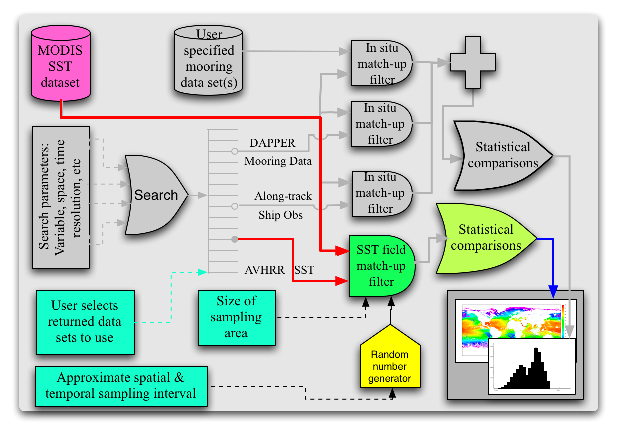
It is not the current version, and thus it cannot be edited. Field Comparison WorkflowThe overall idea of this sequence is to statistically compare two or more SST data sets. The data sets are assumed to consist of 2D SST fields in time; i.e., each field is a lat, lon field, one for each instant in time, with many time steps. (This workflow compromises the colored elements of the modified ocean use (Figure 1) shown in the proposal.) Although this workflow is designed to compare SST fields, it should work for many geo-based arrays.
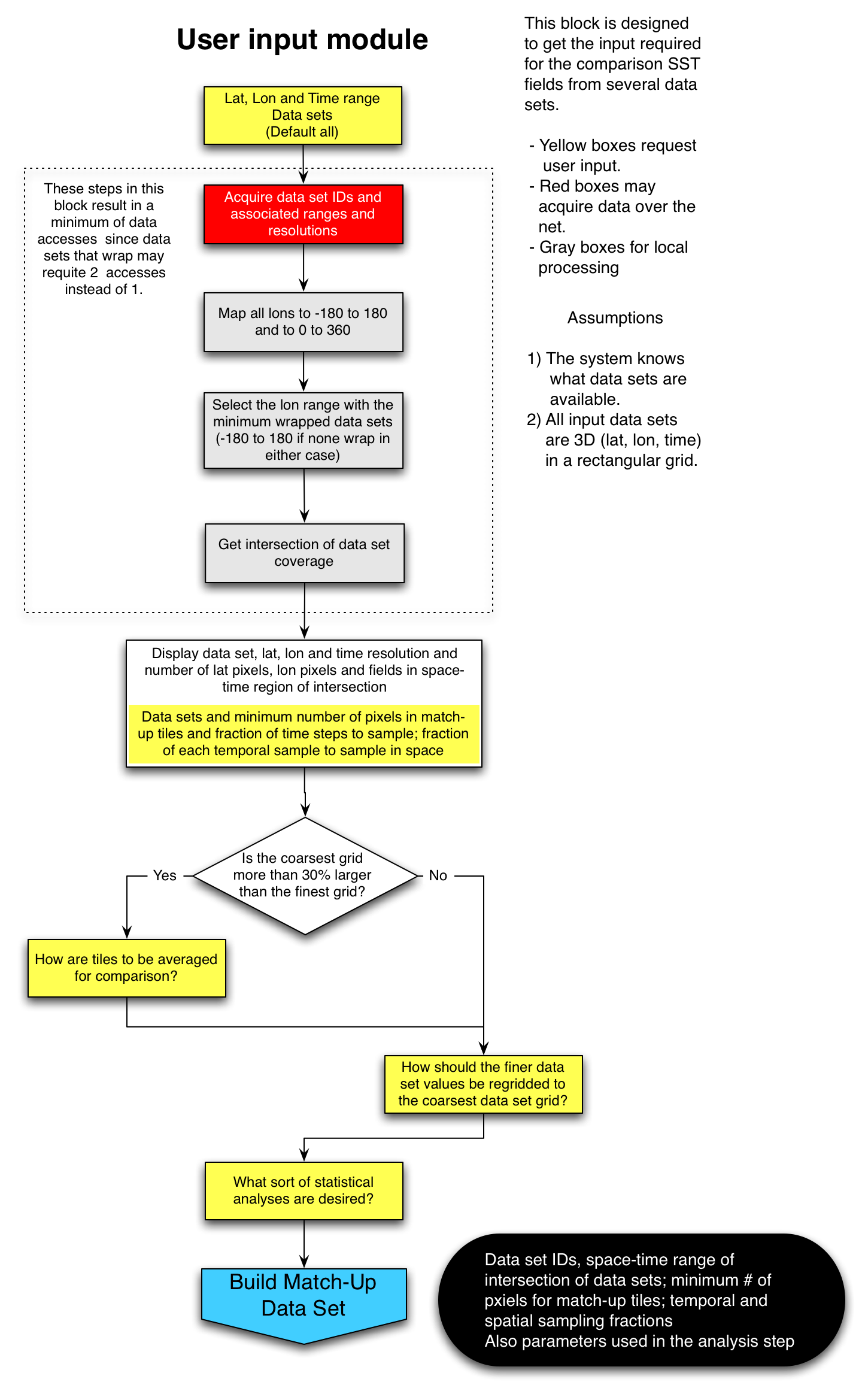
SST fields could be compared point-by-point, but for many data sets this would result in a VERY LARGE computational problem. The solution adopted here for large data sets is to randomly sample the fields in space and time and then to compare samples statistically. The user, based on data set characteristics, specifies the fractions in space and time of the data sets that are to be sampled. The selection process is outlined in the User Input Module. The data sets are then randomly sampled based on these fractions. An additional complication is that the grid spacing may differ between data sets. In order to address this, the size of each sample is based on the area of the coarsest grid; i.e, the area sampled for each data set will be the same, but the number of samples will not be. Sampling is described in the Build Match-Up Data Set Module. In the analysis phase decisions must be made on how to compare arrays of different size. These decisions will be made interactively with the user and are discussed in the Analysis Module. Initially, the comparison simply provides mean and standard deviation of the differences. Later, one could imagine filtering the results by space and time. For example, suppose that the user wants to compare a 25km AMSR-E SST data set with a 4km MODIS SST data set. (This example - use case - to be fleshed out in more detail.) 1) User Input Module (Figure 2 below.) The first block of this module requests lat, lon, time ranges from the user as well as data sets of interest. This could be done iteratively - the user specifies lat, lon, time, variable and resolution ranges and the system returns a list of data sets from which the user selects those of interest. The module then gets the metadata associated with data sets that meet the user's request. Because longitude can be specified on any 360 degree interval, it is possible that the ranges of data sets will not coincide. This could result in additional unnecessary requests when performing the subsampling that is required by subsequent module. For example, one may go from -180 to 180 and another from 0 to 360. When requesting data, if a user is interested in data between 170 and 190, these data would in general be accessible via one request (in time) for the 0 to 360 data set, but 2 requests for the -180 to 180 data set. In order to minimize, or preferably eliminate, the number of multiple requests from the same field, the next several blocks of code find the longitude range that minimizes the number of `wrapped' data sets. Once the data sets have been selected, their metadata is acquired and the need for additional input determined. First, the module requests of the user parameters to be used in the random sampling of the arrays for comparison. Next the module determines if the grid sizes are very different, defined here as 30%. If they are, then some sort of averaging of the finer grids up to the coarser grid size may be desired. The user is queried for these parameters. Finally, the user is asked what sort of statistical analyses are to be performed.
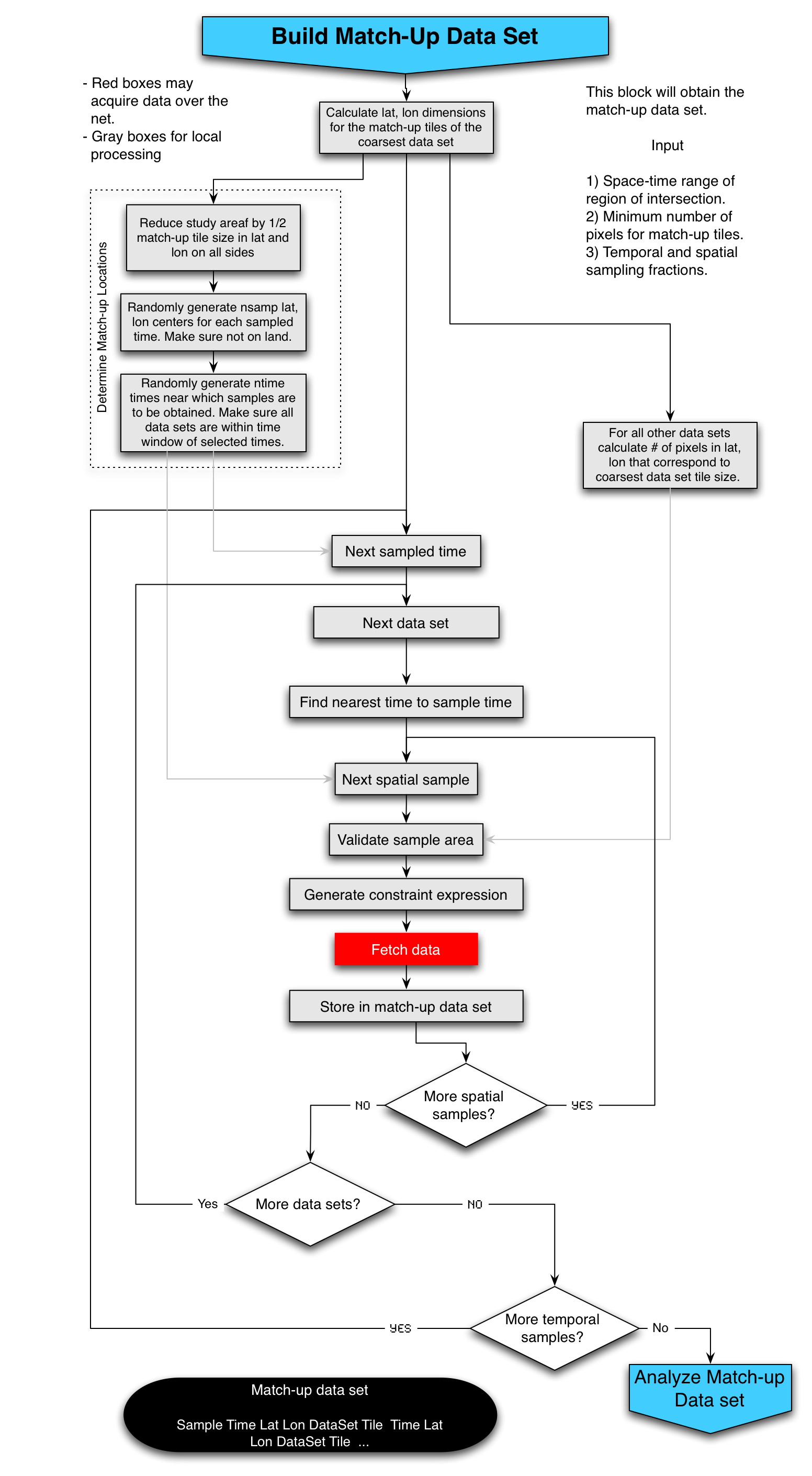
2) Build Match-Up Data Set Module (Figure 3 below.) This block calculates where in space and time the samples are to be taken, the size of the area to be sampled for each data set and then acquires the samples and stores them in a match-up data base. The areas to be sampled are based on the size of the coarsest data set and the minimum number of pixels per sample passed in from the User Input Module. The first block in this module calculates this area and from that the number of grid elements in all other modules based on this area. The second block, labeled Determine Match-up Locations randomly determines the spatial and temporal location of the center of tiles for which match-up tuples will be obtained. In parallel with this, the size of tiles in each of the other data sets is calculated. Because the type of project may be different from data set to data set, care will have to be taken at this point to make sure that the sample areas in the finer data sets cover the coarser sample area at all latitudes. This may require the sample area being calculated at a later step (just prior to generating the constraint expression) for some data sets. This should be determined at this point. ' Following generation of the location in space and time of the samples, there are three loops, one over time, the second over data sets and the third over space. The reason for this ordering of loops is that most SST data sets are currently 2D (longitude, latitude) fields in time. Also there will generally be many spatial samples for each temporal field sampled. So the module gets a field at a given time for the first data set, acquires all of the spatial samples for this time, data set pair, then goes to the next data set finding the nearest time and repeats until all data sets have been sampled, then it goes to the next instance in time. The output of this module is the Match-up Data Set which consists of time, space, SST tile tuples:
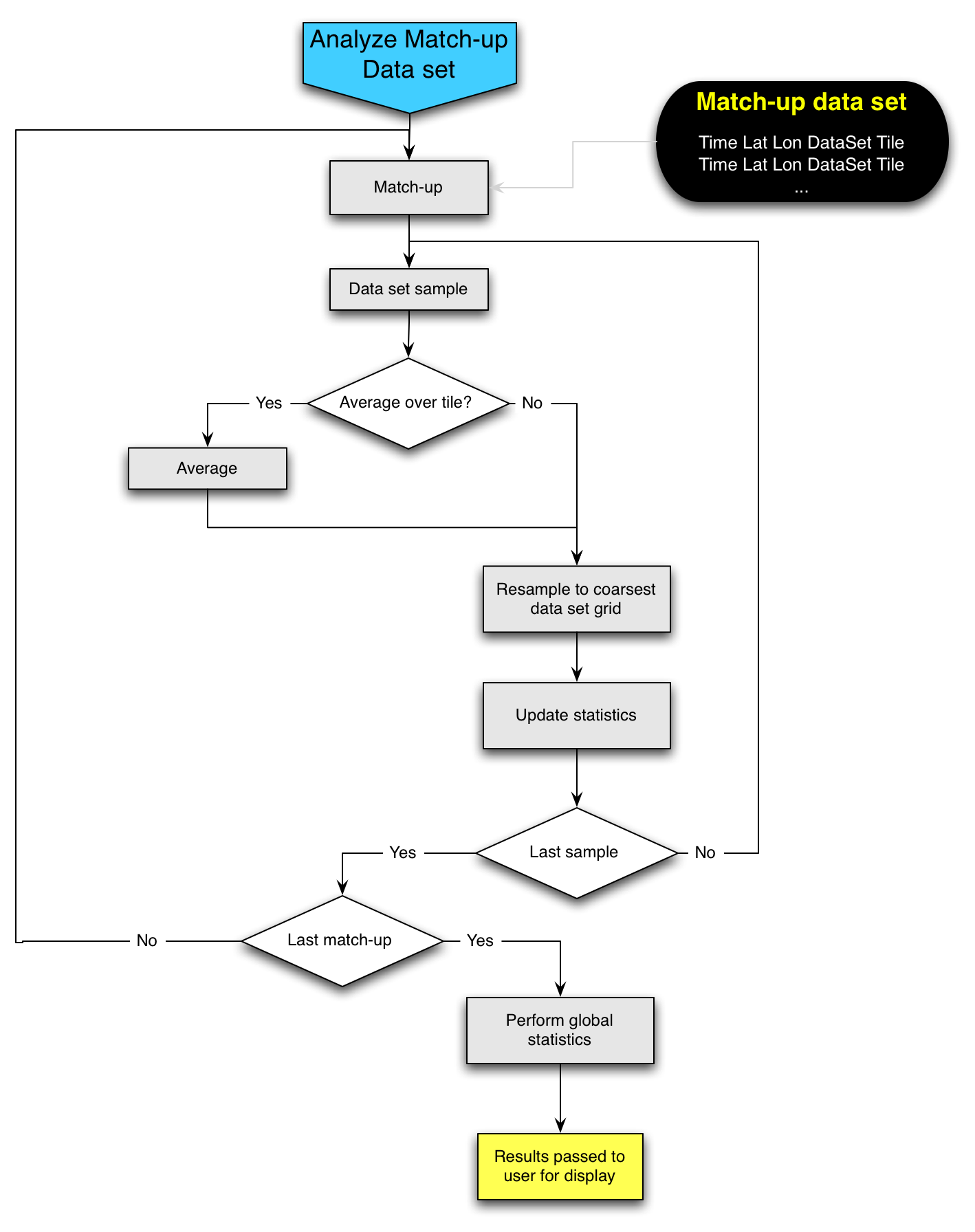
3) Analysis Module (Figure 4 below.) In this module the Match-up Data Set is analyzed. The module consists of two main loops, one over match-ups and the second, inner loop, over data set tiles within a match-up. The basic idea is to gather statistics for each time in each match-up and to statistically compare these as a function of space, time, data set, etc. All tiles are referenced to the grid of the coarsest data set. For finer data sets, the data are averaged up if necessary and then resampled to the coarsest grid, again if necessary. Whether or not to average and regrid is determined by the user via input in the User Input Module. Once averaging and regridding has been performed for a tile, the statistics associated with the tile are calculated. At the outset, these statistics will be sum of SSTs, sum of squares, and number of good values in the tile and similar values for the differences between this data set and all of the other data sets that have been examined for this match-up to this point in the loop. (This way, all pairs will be calculated with no repetition.) Once all of the match-ups have been processed, control passes out of the loops to a block that calculates global statistics for the data base. This data set is then exposed to the user for plotting, tabulating, etc. This data set will consist of:
From this data set the user may calculate mean, sigma for all of the differences and each grid. This can be done globally, by match-up sample or by samples falling in a given space-time region. The user may also stratify by data set. There are of course higher order statistics that some may want to calculate, but I think that these simple stats will keep us busy.
ACTION ITEMS AND FUTURE STEPS FROM THE SST BREAK OUT
Attachments:
|
| This material is based upon work supported by the National Science Foundation under award 0619060. Any opinions, findings and conclusions or recomendations expressed in this material are those of the author(s) and do not necessarily reflect the views of the National Science Foundation (NSF). Copyright 2007 |